Intro to Statistical methods using RStudio




Page 1: Data handling and descriptive statistics,
Page 2: Probability,
Page 3: Intervals and sample size,
Page 4: Hypothesis Testing,
Page 5: Contingency tables,
Page 6: Linear Regression.

Page 1: Data handling and descriptive statistics

0. Handing datasets in R

# Basic handling of datasets
# R datasets from base R packages, example:
data(mtcars)
head(mtcars)
#to see the list of all dataset available in R, run
data()

# from an specific package, kid.weights from UsingR
require(UsingR)
head(kid.weights)

#vectors (one variable)
my_data <- c(1,2,3,4,5,6,7,8)

#downloading directly from a website, URL known: fread(url)
install.packages("data.table")
library(data.table)
babywght <- fread("http://jse.amstat.org/datasets//babyboom.dat.txt")
# Dataset description http://jse.amstat.org/datasets/babyboom.txt
head(babywght,3) # dataset head, first 3 rows.

#OR reading from directory:
#go to Environment > import Dataset or # go to Files, click on a Dataset

#writing (saving) to directory.
#Set directory at Tools > Global Options > Default Working Directory
# what is the current directory?
getwd()
# mine:
#"C:/Users/csotu/Documents/R"
#-- this is the PATH #Export or save dataset on your directory as csv file:
library("writexl")
#"C:/Users/csotu/Documents/R" -- taken from getwd()
# format: write_csv(dataset, "path\\dataset.csv") # for example:
write_csv(kid.weights, "C:\\Users\\csotu\\OneDrive\\Documents\\R\\data_files\\kid.weights.csv")

# structure of Dataset.
Function str base R or glimpse, from dplyr:
str(mtcars)
require(dplyr)
glimpse(mtcars)

dim(mtcars)# it just yields number of rows by colns
names(mtcars) # it just yields columns' names (variables)
head(mtacrs) # first six observations (rows)
tail(mtcars) # bottom six observations (rows)

# is there missing data (NAs) ? # NAs
sum(is.na(my.dataset)) # NAs in total
colSums(is.na(my.dataset)) # by columns
colSums(is.na(mtcars)) # none
colSums(is.na(airquality)) # several: airquality is a base R Dataset

# changing variables from numeric (double) to categorical (factor)
mtcars$cyl<-as.factor(mtcars$cyl) # in base R
str(mtcars)
#or
library(dplyr)
df <- df %>% mutate_at(c('var1', 'var2'), as.factor) #general format
mtcars <- mtcars %>% mutate_at(c("cyl", "vs", "am"), as.factor)# example
str(mtcars)

1. Basic descriptive statistics

#sample of McDonald waiting time in secs:

waiting_McD <- c(83,90,91,100,101,107,113,117,117,119,123,127,127,127,130,133, 135,138,139,140,143,144,144,148,150,151,153,153,154,155,163,167,169,169,171,184,
186,187,190,196,197,197,200,206,209,252, 254,255,281,308)

length(waiting_McD)
summary(waiting_McD)

install.packages("modeest")
library(modeest)
mlv(waiting_McD,method="mfv")

#or, Mode in DescTools
install.packages("DescTools")
library(DescTools)
Mode(waiting_McD)

sample.mean <- sum(waiting_McD)/length(waiting_McD)
sample.mean
mean(waiting_McD)
var((waiting_McD)
sd((waiting_McD)

install.packages("psych")
library(psych)
describe((waiting_McD)

# creating classes on a numeric variable:
classes <- cut(x = waiting_McD, breaks=c(80,124, 174,224,274,324), right=F)
TB <- table(classes)
TB1 <- as.data.frame(TB); TB1
rel.fr <- (TB1$Freq)/50
TB2 <- cbind(TB1,rel.fr);TB2

#OR
require(dplyr)
TB2 <- TB1 %>% mutate(rel.frq=Freq/50) %>% as.data.frame(); TB2
TB3 <- TB1 %>% mutate(cum.frq=cumsum(Freq)) %>% as.data.frame(); TB3

install.packages("knitr")
require(knitr)
TB3i <- kable(TB3) TB3i # a better looking table

# Applying functions to a variable (column) in a dataset:
#Base R, example (one function)
mean(mtcars$mpg)
# by a factor (say cyl, in mtcars), using aggregate in base R:
group_mean <- aggregate(mpg ~ cyl, data = mtcars, mean);group_mean
groups_mean <- aggregate(mpg ~ cyl+am, data = mtcars, mean);groups_mean
# create a function of functions:
afun<-function(x){c(mean=mean(x), sd=sd(x), median=median(x))}
group_funs <- aggregate(mpg ~ cyl, data = mtcars,afun);group_funs
# Using dplyr package
require(dplyr)
mtcars%>%group_by(cyl)%>%summarize(mean_mpg=mean(mpg), median_mpg=median(mpg), sd_mpg=sd(mpg))%>%as.data.frame()
# dplyr: creating a function of functions, as needed:
my.fun <- function(x) {c(min = min(x), mean = mean(x), std=sd(x), max = max(x))}
mtcars%>%dplyr::select(mpg, hp, wt)%>%apply(MARGIN=2, FUN=my.fun)

2. Histograms:

# 40 human males heights dataset. Entering the data as a vector:
heights40 <- c(187,171,181,180,178,171,174,177,172,178,182,187,176,179,190,185, 192,184,182,178,187,173,185,184,184,183,185,197,202,181,181,191, 178,187,185,186,174,174,182,195)

length(heights40)
hist(heights40, xlab="Heights of 40 men in cm", main="Histogram")
hist(heights40, freq=FALSE, col = 'lightblue', xlab="Heights of 40 men in cm", main="Histogram")
lines(density(heights40))

#using ggplot, hist of temp dataset airquality (base R)
airquality%>%drop_na()%>%ggplot(aes(x=Temp))+geom_histogram(fill=I("lightblue"))

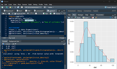
# for the base R dataset rivers.
rivers <- as.data.frame(rivers)
ggplot(rivers, aes(rivers))+geom_histogram(aes(y = ..density..))
ggplot(rivers, aes(rivers))+stat_density()

# for height40 on ggplot:
heights40 <- as.data.frame(heights40)
ggplot(heights40, aes(heights40))+geom_histogram(aes(y = ..density..))
ggplot(heights40, aes(heights40))+stat_density()

3. Barplots:

# Survey: what is your favorite color:
#Entering data in base R, firtly, as vectors:
colors <- c("Blue", "Green", "Purple", "Red", "Other")
Percent <- c(37,25,17,15,6)
# create a data frame from the vectors:
fav.col <- data.frame(colors,Percent)
kable(fav.col)
with(fav.col, barplot(Percent, names.arg=colors))

require(dplyr)
head(mtcars,3)
mtcars$am <- recode(mtcars$am, "0" = "auto","1"="manual")
# instead, you may use "ífelse" as follows:
mtcars<-mtcars%>%mutate(am=ifelse(am==0,"auto","manual"))
head(mtcars)
table2<-xtabs(~cyl+am, data=mtcars);table2
barplot(table2, legend.text=T)
table4<-xtabs(~am+cyl, data=mtcars);table4
barplot(table4, legend.text=T, xlab="num of cyls")
barplot(table4, legend.text=T, beside=T,xlab="num of cyls")

#Using ggplot2 package
require(ggplot2)
ggplot(fav.col, aes(x = colors, y = Percent)) + geom_col() + geom_text(aes(label = Percent), vjust = 1.5, colour = "white")
ggplot(mtcars, aes(x=vs))+geom_bar()+ geom_text(aes(label=..count..),stat= "count", vjust=-0.25)

4. Stem and Leaf Plots:

the.data <- c( 12, 23, 19, 16, 10, 17, 15, 25, 21, 12, 30, 32, 45)
stem(x=the.data, scale = 1)
# for height40
stem(x=heights40, scale = 0.5) # sort(heights40) & compare...
sort(heights40)

5. Boxplots:

install.packages("UsingR")
install.packages("psych")
library(UsingR)
library(psych)
head(normtemp) # https://jse.amstat.org/datasets/normtemp.txt
dim(normtemp)
describe(temperature~gender, fast=T, data=normtemp)
boxplot(temperature~gender, data=normtemp)

# mpg by cylinders
describe(mpg~cyl, fast=T, data=mtcars)
boxplot(mpg~cyl, fast=T, data=mtcars)

#Using ggplot2
library(ggplot2)
ggplot(data = mtcars, aes(x = factor(cyl), y = mpg )) +
geom_boxplot(fill = "gray") +
ggtitle("Distribution of Gas Mileage") +
ylab("MPG") +
xlab("Cylinders")

6. QQ-plots:

# QQ plots
head(kid.weights,3) # for a data.frame
with(kid.weights, qqnorm(height, pch = 1))
with(kid.weights, qqline(height, col = "steelblue", lwd = 2))

heights40 <- c(187,171,181,180,178,171,174,177,172,178,182,187,176,179,190,185, 192,184,182,178,187,173,185,184,184,183,185,197,202,181,181,191, 178,187,185,186,174,174,182,195)

# qq plot for a vector in base R
qqnorm(heights40, pch = 1)
qqline(heights40, col = "steelblue", lwd = 2)