Intro to Statistical methods using RStudio





Page 1: Data handling and descriptive statistics,
Page 2: Probability,
Page 3: Intervals and sample size,
Page 4: Hypothesis Testing,
Page 5: Contingency tables,
Page 6: Linear Regression.

Page 6: Linear Regression,

0. Linear regression analysis:

Linear regression analysis is used to predict the value of a variable based on the value of another variable

1. Testing assumptions:

#Linearity: The relationship between X and the mean of Y is linear. #Homoscedasticity: The variance of residual is the same for any value of X.
#Independence: Observations are independent of each other.
#Normality: For any fixed value of X, Y is normally distributed.

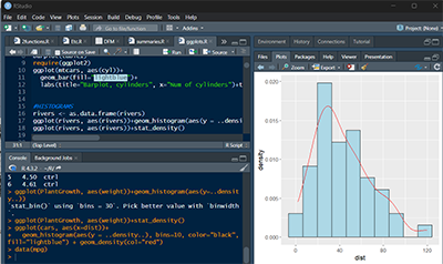
# linear regression
require(UsingR)
head(heartrate)
dim(heartrate)
plot(heartrate)

#model model1 <- lm(maxrate~age, data=heartrate)
summary(model1)
par(mfrow = c(2, 2))
plot(model1)

2. Interpreting output of plot(model):

#the residual vs fitted plot will show no fitted pattern. That is, the red line should be
#approximately horizontal at zero. The presence of a pattern may indicate a problem
#with some aspect of the linear model.
#Homogeneity of variance #This assumption can be checked by examining the scale-location plot,
#also known as the spread-location plot.
# It’s good if you see a horizontal line with equally spread points.
#Normality of residuals
# The normal probability plot (QQ residuals)
#of residuals should approximately follow a straight line.
# A residuals vs. leverage plot is a type of diagnostic plot
#that allows us to identify influential observations in a regression model.

3. Another example:

head(cars,3)
dim(cars)
summary(cars)
boxplot(cars)
with(cars, qqnorm(speed))
with(cars, qqnorm(dist))
model2 <- lm(dist~speed, data=cars)
summary(model2)
plot(model2)

4. Correlation:

Correlation is a statistical measure that expresses the extent to which two variables are linearly related (meaning they change together at a constant rate).
The cor() function will calculate the correlation between two vectors:

#correlation coefficient:
with(cars, cor(dist,speed))

Possible values of the correlation coefficient range from -1 to +1, with -1 indicating a perfectly linear negative, i.e., inverse, correlation (sloping downward) and +1 indicating a perfectly linear positive correlation (sloping upward). A correlation coefficient close to 0 suggests little, if any, correlation