Example 1: Use a two-sample t-test to determine whether the unknown population means of newborns' weight is the same for both sex.

Data:
NAME: Time of Birth, Sex, and Birth Weight of 44 Babies
TYPE: Observational
SIZE: 44 observations, 4 variables

DESCRIPTIVE ABSTRACT:
The dataset contains the time of birth, sex, and birth weight for each of 44 babies born in one 24-hour period at a Brisbane, Australia, hospital.  Also included is the number of minutes since midnight for each birth.

Dataset description http://jse.amstat.org/datasets/babyboom.txt

Dataset: http://jse.amstat.org/datasets/babyboom.dat.txt

Downloading data from URL using the fread from data.table package:

install.packages("data.table")
library(data.table)

Storing the data as object babywght:

babywght <- fread("http://jse.amstat.org/datasets//babyboom.dat.txt")

How many rows (observations) and columns (variables) on the dataset?

dim(babywght) # dataset dimensions rows by columns
[1] 44  4
head(babywght,3) # dataset head, first 3 rows.

...  V1 V2   V3 V4
1:   5  1 3837  5
2: 104  1 3334 64
3: 118  2 3554 78

By the description of the dataset we learn that the name of the variables are:
Time, Sex, Weight in grams and Minutes after midnight.
Selecting V2, Sex and V3, Weight in grams.

babywght <- babywght %>% select(V2, V3) # or in base R:
babywght <- babywght[,c(-1,-4)]
head(babywght,3)

...V2 V3
1: 1 3837
2: 1 3334
3: 2 3554

Naming the two variables of interest: Sex and Weight:

names(babywght) <- c("Sex", "Weight(g)")
head(babywght)   

....Sex Weight(g)
1:   1      3837
2:   1      3334
3:   2      3554

Structure:

str(babywght)

Classes ‘data.table’ and 'data.frame':       44 obs. of  2 variables:
 $ Sex      : int  1 1 2 2 2 1 1 2 2 2 ...
 $ Weight(g): int  3837 3334 3554 3838 3625 46 3166 3520 ...

Convert the numeric variable into a factor.
Recode Sex 1 as Female, and 2 as Male according to the dataset description:

babywght$Sex <- as.factor(babywght$Sex)
babywght <-babywght %>% mutate(Sex=if_else(Sex=="1", "F", "M"));head(babywght,3)

....Sex Weight(g)
1:   F      3837
2:   F      3334
3:   M      3554

Rename the variable Weight(g) as just Weight, using dplyr in order to simplify the variable's name:

babywght <- babywght %>% rename(Weight=`Weight(g)`)
head

....Sex Weight
1:   F   3837
2:   F   3334

The Study begins now. A table by Sex:

table1 <- babywght %>% count(Sex);table1  

....Sex  n
1:   F 18
2:   M 26

Descriptive statistics by Sex: mean, median, standard deviation, minimun and maximun values:

babywght %>% group_by(Sex) %>% summarise_all(list(mean=mean,median=median, sd=sd, min=min,max=max))

.Sex    mean median    sd   min   max
<chr> <dbl>  <dbl> <dbl> <int> <int>
1 F     3132.   3381  632.  1745  3866
2 M     3375.   3404  428.  2121  4162

Boxplots using ggplot2 package:

require(ggplot2)
ggplot(babywght,aes(x=Sex,y=Weight))
+geom_boxplot()+theme_dark()

Output:

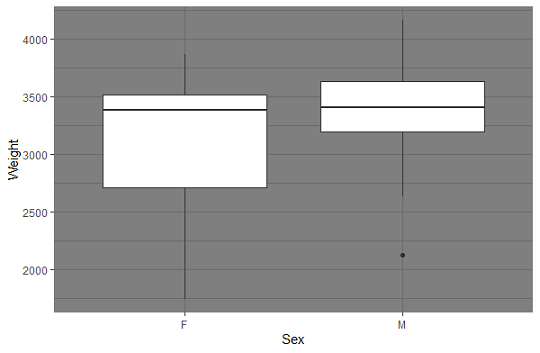
The median weight es quite similar for both groups; the variation is much larger among females. There is an outloier in the Male group.

with(babywght, shapiro.test(Weight[Sex=="M"]))

Shapiro-Wilk normality test
data:  Weight[Sex == "M"]
W = 0.947= 0.2022

with(babywght, shapiro.test(Weight[Sex=="F"]))

Shapiro-Wilk normality test
data:  Weight[Sex == "F"]
W = 0.87028, p-value = 0.01798

Conclusion: Normality based on the Shapiro test cannot not be rejected for the males'group. For the females'group, however, normality is rejected at about 1.8%. Notice that there are only 18 data points for the females'group.
A larger sample size may be needed.

2. Assessing homogeneity of variances:

ftest <- var.test(Weight ~ Sex, data = babywght);ftest

F test to compare two variances
data:  Weight by Sex
F = 2.1771, num df = 17, denom df = 25, p-value = 0.07526
alternative hypothesis: true ratio of variances is not equal to 1
95 percent confidence interval:
 0.9225552 5.5481739
sampl
ratio of variances
          2.177104

Conclusion: With a p-value of 0.075 we fail to reject the equality of variances.

Testing...

Let's conduct a non-parametric test first considering that normality for the females group is in doubt.

Wilcox.test(Weight ~ Sex, data = babywght, alternative = "two.sided")

Wilcoxon rank sum test with continuity correction
data:  Weight by Sex
W = 194.5, p-value = 0.3519
alternative hypothesis: true location shift is not equal to 0

Parametric test:

t.test(Weight ~ Sex, data=babywght, Paired= F, var.equal=TRUE)

               Two Sample t-test
data:  Weight by Sex
t = -1.5229, df = 42, p-value = 0.1353
alternative hypothesis: true difference in means between group F and group M is not equal to 0
95 percent confidence interval:
 -564.70440   78.97791
sample estimates:
mean in group F mean in group M
       3132.444        3375.308

Conclusions:
Both, the non-parametric and the parametric tests tell us that there is no significant difference between the mean weight for newborn girls and boys born on given day at a hospital in Australia.